Quantum computing harnesses the principles of quantum mechanics to perform computations in fundamentally different ways than classical computers. At the heart of quantum computing is linear algebra, which provides the mathematical framework for understanding and manipulating quantum states. This guide will introduce you to the essential concepts of linear algebra that are crucial for quantum computing.
In quantum computing, the state of a quantum system is represented by a vector in a complex vector space known as a Hilbert space.
The simplest definition of vectors and matrices is as follows.
A single row of numbers is called a vector.
A single column of numbers is also called a vector.
A grid of numbers (with multiple rows and columns) is called a matrix.
These definitions suffice to explain how to perform several different operations involving vectors and matrices.
In quantum computing, the state of the qubits is represented by a vector. The logic gates of a quantum circuit can be written as matrices. The measurement operators that output the results of the computation can also be written as matrices. More broadly, vectors and matrices permeate the fields of machine learning, data analysis and many other technical domains.
The basics of vectors and matrices can be studied with minimal mathematical background. The insights they provide a very useful for going deeper into quantum computing.
For a single qubit, the state is a vector in a two-dimensional Hilbert space, typically denoted as ∣ψ⟩. The basis vectors of this space are ∣0⟩ and ∣1⟩, corresponding to the classical bit values 0 and 1.
A general qubit state can be written as:
∣ψ⟩=α∣0⟩+β∣1⟩
where α and β are complex numbers satisfying:
∣α∣²+∣β∣²=1.
Dirac notation, or bra-ket notation, is a concise way to represent quantum states. The vector ∣ψ⟩ is called a ket, and its conjugate transpose ⟨ψ∣ is called a bra. Inner products (dot products) are written as ⟨ϕ∣ψ⟩, and outer products are written as ∣ψ⟩⟨ϕ∣.
Quantum operations are represented by linear operators, which are matrices acting on the state vectors. Common operators include:
Pauli Matrices: Represent basic quantum gates.
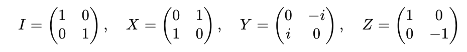
Hadamard Gate: Creates superposition.

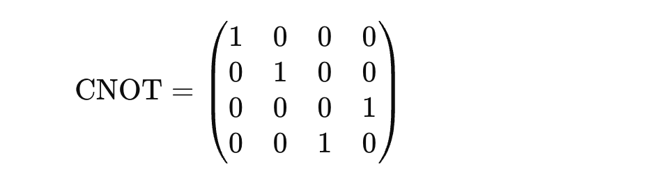
Controlled-NOT (CNOT) Gate: Entangles qubits.
Operators have eigenvalues and eigenvectors, which are essential for understanding measurement in quantum mechanics. If A is an operator, then ∣ψ⟩ is an eigenvector of A with eigenvalue λ if:
A∣ψ⟩=λ∣ψ⟩
In quantum computing, measuring a state corresponds to projecting it onto an eigenvector of the measurement operator, collapsing the state to that eigenvector and returning the eigenvalue as the measurement result.
Quantum systems with multiple qubits are described using tensor products. If ∣ψ⟩ is a state of qubit 1 and ∣ϕ⟩ is a state of qubit 2, the combined state is: ∣ψ⟩⊗∣ϕ⟩.
For example, if ∣ψ⟩=α∣0⟩+β∣1⟩ and ∣ϕ⟩=γ∣0⟩+δ∣1⟩, then:
∣ψ⟩⊗∣ϕ⟩=αγ∣00⟩+αδ∣01⟩+βγ∣10⟩+βδ∣11⟩.
Quantum evolution is governed by unitary transformations, which are matrices U satisfying U†U = I, where U† is the conjugate transpose of U. Unitarity ensures that the length (norm) of the state vector is preserved, maintaining the probabilistic interpretation of quantum states.
Measurement in quantum computing collapses the state vector to one of the basis states, with probabilities given by the squared absolute values of the coefficients. For a state ∣ψ⟩=α∣0⟩+β∣1⟩, the probability of measuring ∣0⟩ is ∣α∣² and ∣1⟩ is ∣β∣²
Linear algebra forms the backbone of quantum computing, providing the tools to describe and manipulate quantum states and operations. Understanding vectors, matrices, eigenvalues, tensor products, unitary transformations, and measurement is essential for anyone venturing into the world of quantum computation. This mathematical framework enables the profound capabilities of quantum computers, offering the potential to solve problems beyond the reach of classical computing.